Parent classes¶

There are many different cases which might be desirable for fitting an IMNN, i.e. generating simulations on-the-fly with SimulatorIMNN(), or with a fixed set of analytic gradients with GradientIMNN() or performing numerical gradients for the derivatives with NumericalGradientIMNN(), or when the datasets are very large (either in number of elements - n_s - or in shape - input_shape) then the gradients can be manually aggregated using AggregatedSimulatorIMNN(), imnn.AggregatedGradientIMNN() or AggregatedNumericalGradientIMNN(). These are all wrappers around a base class _IMNN() and optionally an aggregation class _AggregatedIMNN(). For completeness these are documented here.

The available modules are:

Base class
Aggregation of gradients

Base class ¶

class imnn.imnn._imnn._IMNN(n_s, n_d, n_params, n_summaries, input_shape, θ_fid, model, optimiser, key_or_state)¶

Information maximising neural network parent class

This class defines the general fitting framework for information maximising neural networks. It includes the generic calculations of the Fisher information matrix from the outputs of a neural network as well as an XLA compilable fitting routine (with and without a progress bar). This class also provides a plotting routine for fitting history and a function to calculate the score compression of network outputs to quasi-maximum likelihood estimates of model parameter values.

The outline of the fitting procedure is that a set of \(i\in[1, n_s]\) simulations and \(n_d\) derivatives with respect to physical model parameters are used to calculate network outputs and their derivatives with respect to the physical model parameters, \({\bf x}^i\) and \(\partial{{\bf x}^i}/\partial\theta_\alpha\), where \(\alpha\) labels the physical parameter. The exact details of how these are calculated depend on the type of available data (see list of different IMNN below). With \({\bf x}^i\) and \(\partial{{\bf x}^i}/\partial\theta_\alpha\) the covariance

\[C_{ab} = \frac{1}{n_s-1}\sum_{i=1}^{n_s}(x^i_a-\mu^i_a) (x^i_b-\mu^i_b)\]

and the derivative of the mean of the network outputs with respect to the model parameters

\[\frac{\partial\mu_a}{\partial\theta_\alpha} = \frac{1}{n_d} \sum_{i=1}^{n_d}\frac{\partial{x^i_a}}{\partial\theta_\alpha}\]

can be calculated and used form the Fisher information matrix

\[F_{\alpha\beta} = \frac{\partial\mu_a}{\partial\theta_\alpha} C^{-1}_{ab}\frac{\partial\mu_b}{\partial\theta_\beta}.\]

The loss function is then defined as

\[\Lambda = -\log|{\bf F}| + r(\Lambda_2) \Lambda_2\]

Since any linear rescaling of a sufficient statistic is also a sufficient statistic the negative logarithm of the determinant of the Fisher information matrix needs to be regularised to fix the scale of the network outputs. We choose to fix this scale by constraining the covariance of network outputs as

\[\Lambda_2 = ||{\bf C}-{\bf I}|| + ||{\bf C}^{-1}-{\bf I}||\]

Choosing this constraint is that it forces the covariance to be approximately parameter independent which justifies choosing the covariance independent Gaussian Fisher information as above. To avoid having a dual optimisation objective, we use a smooth and dynamic regularisation strength which turns off the regularisation to focus on maximising the Fisher information when the covariance has set the scale

\[r(\Lambda_2) = \frac{\lambda\Lambda_2}{\Lambda_2-\exp (-\alpha\Lambda_2)}.\]

Once the loss function is calculated the automatic gradient is then calculated and used to update the network parameters via the optimiser function. Note for large input data-sizes, large \(n_s\) or massive networks the gradients may need manually accumulating via the _AggregatedIMNN().

_IMNN is designed as the parent class for a range of specific case IMNNs. There is a helper function (IMNN) which should return the correct case when provided with the correct data. These different subclasses are:

SimulatorIMNN():

Fit an IMNN using simulations generated on-the-fly from a jax (XLA compilable) simulator

GradientIMNN():

Fit an IMNN using a precalculated set of fiducial simulations and their derivatives with respect to model parameters

NumericalGradientIMNN():

Fit an IMNN using a precalculated set of fiducial simulations and simulations generated using parameter values just above and below the fiducial parameter values to make a numerical estimate of the derivatives of the network outputs. Best stability is achieved when seeds of the simulations are matched between all parameter directions for the numerical derivative

AggregatedSimulatorIMNN():

SimulatorIMNN distributed over multiple jax devices and gradients aggregated manually. This might be necessary for very large input sizes as batching cannot be done when calculating the Fisher information matrix

AggregatedGradientIMNN():

GradientIMNN distributed over multiple jax devices and gradients aggregated manually. This might be necessary for very large input sizes as batching cannot be done when calculating the Fisher information matrix

AggregatedNumericalGradientIMNN():

NumericalGradientIMNN distributed over multiple jax devices and gradients aggregated manually. This might be necessary for very large input sizes as batching cannot be done when calculating the Fisher information matrix

DatasetGradientIMNN():

AggregatedGradientIMNN with prebuilt TensorFlow datasets

DatasetNumericalGradientIMNN():

AggregatedNumericalGradientIMNN with prebuilt TensorFlow datasets

There are currently two other parent classes

AggregatedIMNN():

This is the parent class which provides the fitting routine when the gradients of the network parameters are aggregated manually rather than automatically by jax. This is necessary if the size of an entire batch of simulations (and their derivatives with respect to model parameters) and the network parameters and their calculated gradients is too large to fit into memory. Note there is a significant performance loss from using the aggregation so it should only be used for these large data cases

Parameters

n_s (int) – Number of simulations used to calculate network output covariance
n_d (int) – Number of simulations used to calculate mean of network output derivative with respect to the model parameters
n_params (int) – Number of model parameters
n_summaries (int) – Number of summaries, i.e. outputs of the network
input_shape (tuple) – The shape of a single input to the network
θ_fid (float(n_params,)) – The value of the fiducial parameter values used to generate inputs
validate (bool) – Whether a validation set is being used
simulate (bool) – Whether input simulations are generated on the fly
_run_with_pbar (bool) – Book keeping parameter noting that a progress bar is used when fitting (induces a performance hit). If run_with_pbar = True and run_without_pbar = True then a jit compilation error will occur and so it is prevented
_run_without_pbar (bool) – Book keeping parameter noting that a progress bar is not used when fitting. If run_with_pbar = True and run_without_pbar = True then a jit compilation error will occur and so it is prevented
F (float(n_params, n_params)) – Fisher information matrix calculated from the network outputs
invF (float(n_params, n_params)) – Inverse Fisher information matrix calculated from the network outputs
C (float(n_summaries, n_summaries)) – Covariance of the network outputs
invC (float(n_summaries, n_summaries)) – Inverse covariance of the network outputs
μ (float(n_summaries,)) – Mean of the network outputs
dμ_dθ (float(n_summaries, n_params)) – Derivative of the mean of the network outputs with respect to model parameters
state (:obj:state) – The optimiser state used for updating the network parameters and optimisation algorithm
initial_w (list) – List of the network parameters values at initialisation (to restart)
final_w (list) – List of the network parameters values at the end of fitting
best_w (list) – List of the network parameters values which provide the maxmimum value of the determinant of the Fisher matrix
w (list) – List of the network parameters values (either final or best depending on setting when calling fit(…))
history (dict) –
A dictionary containing the fitting history. Keys are
- detF – determinant of the Fisher information at the end of each iteration
- detC – determinant of the covariance of network outputs at the end of each iteration
- detinvC – determinant of the inverse covariance of network outputs at the end of each iteration
- Λ2 – value of the covariance regularisation at the end of each iteration
- r – value of the regularisation coupling at the end of each iteration
- val_detF – determinant of the Fisher information of the validation data at the end of each iteration
- val_detC – determinant of the covariance of network outputs given the validation data at the end of each iteration
- val_detinvC – determinant of the inverse covariance of network outputs given the validation data at the end of each iteration
- val_Λ2 – value of the covariance regularisation given the validation data at the end of each iteration
- val_r – value of the regularisation coupling given the validation data at the end of each iteration
- max_detF – maximum value of the determinant of the Fisher information on the validation data (if available)

model:: Neural network as a function of network parameters and inputs

_get_parameters:: Function which extracts the network parameters from the state

_model_initialiser:: Function to initialise neural network weights from RNG and shape tuple

_opt_initialiser:: Function which generates the optimiser state from network parameters

_update:: Function which updates the state from a gradient

Public Methods:

`__init__`(n_s, n_d, n_params, n_summaries, …)	Constructor method
`fit`(λ, ε[, rng, patience, min_iterations, …])	Fitting routine for the IMNN
`get_α`(λ, ε)	Calculate rate parameter for regularisation from closeness criterion
`set_F_statistics`([w, key, validate])	Set necessary attributes for calculating score compressed summaries
`get_summaries`([w, key, validate])	Gets all network outputs and derivatives wrt model parameters
`get_estimate`(d)	Calculate score compressed parameter estimates from network outputs
`plot`([ax, expected_detF, colour, figsize, …])	Plot fitting history

Private Methods:

`_initialise_parameters`(n_s, n_d, n_params, …)	Performs type checking and initialisation of class attributes
`_initialise_model`(model, optimiser, key_or_state)	Initialises neural network parameters or loads optimiser state
`_initialise_history`()	Initialises history dictionary attribute
`_set_history`(results)	Places results from fitting into the history dictionary
`_set_inputs`(rng, max_iterations)	Builds list of inputs for the XLA compilable fitting routine
`_get_fitting_keys`(rng)	Generates random numbers for simulation generation if needed
`_fit`(inputs, λ=None, α=None[, min_iterations])	Single iteration fitting algorithm
`_fit_cond`(inputs, patience, max_iterations)	Stopping condition for the fitting loop
`_update_loop_vars`(inputs)	Updates input parameters if `max_detF` is increased
`_check_loop_vars`(inputs, min_iterations)	Updates `patience_counter` if `max_detF` not increased
`_update_history`(inputs, history, counter, ind)	Puts current fitting statistics into history arrays
`_slogdet`(matrix)	Combined summed logarithmic determinant
`_construct_derivatives`(derivatives)	Builds derivatives of the network outputs wrt model parameters
`_get_F_statistics`([w, key, validate])	Calculates the Fisher information and returns all statistics used
`_calculate_F_statistics`(summaries, derivatives)	Calculates the Fisher information matrix from network outputs
`_get_regularisation_strength`(Λ2, λ, α)	Coupling strength of the regularisation (amplified sigmoid)
`_get_regularisation`(C, invC)	Difference of the covariance (and its inverse) from identity
`_get_loss`(w, λ, α[, key])	Calculates the loss function and returns auxillary variables
`_calculate_loss`(summaries, derivatives, λ, α)	Calculates the loss function from network summaries and derivatives
`_setup_plot`([ax, expected_detF, figsize])	Builds axes for history plot

_calculate_F_statistics(summaries, derivatives)¶

Calculates the Fisher information matrix from network outputs

If the numerical derivative is being calculated then the derivatives are first constructed. If the mean is to be returned (for use in score compression), this is calculated and pushed to the results tuple. Then the covariance of the summaries is taken and inverted and the mean of the derivative of network summaries with respect to the model parameters is found and these are used to calculate the Gaussian form of the Fisher information matrix.

Parameters

summaries (float(n_s, n_summaries)) – The network outputs
derivatives (float(n_d, n_summaries, n_params)) – The derivative of the network outputs wrt the model parameters. Note that when NumericalGradientIMNN is being used the shape is float(n_d, 2, n_params, n_summaries) which is then constructed into the the numerical derivative in _construct_derivatives.

Returns

F (float(n_params, n_params)) – Fisher information matrix
C (float(n_summaries, n_summaries)) – Covariance of network outputs
invC (float(n_summaries, n_summaries)) – Inverse covariance of network outputs
dμ_dθ (float(n_summaries, n_params)) – The derivative of the mean of network outputs with respect to model parameters
μ (float(n_summaries)) – The mean of the network outputs

Return type

tuple

_calculate_loss(summaries, derivatives, λ, α)¶

Calculates the loss function from network summaries and derivatives

Parameters

summaries (float(n_s, n_summaries)) – The network outputs
derivatives (float(n_d, n_summaries, n_params)) – The derivative of the network outputs wrt the model parameters. Note that when NumericalGradientIMNN is being used the shape is float(n_d, 2, n_params, n_summaries) which is then constructed into the the numerical derivative in _construct_derivatives.
λ (float) – Coupling strength of the regularisation
α (float) – Calculate rate parameter for regularisation from ϵ criterion

Returns

float – Value of the regularised loss function
tuple –
Fitting statistics calculated on a single iteration
- F (float(n_params, n_params)) – Fisher information matrix
- C (float(n_summaries, n_summaries)) – Covariance of network outputs
- invC (float(n_summaries, n_summaries)) – Inverse covariance of network outputs
- Λ2 (float) – Covariance regularisation
- r (float) – Regularisation coupling strength

_check_loop_vars(inputs, min_iterations)¶

Updates patience_counter if max_detF not increased

If the determinant of the Fisher information matrix calculated in a given iteration is not larger than the max_detF calculated so far then the patience_counter is increased by one as long as the number of iterations is greater than the minimum number of iterations that should be run.

Parameters

inputs (tuple) –
- patience_counter (int) – Number of iterations where there is no increase in the value of the determinant of the Fisher information matrix
- counter (int) – While loop iteration counter
- detF (float(max_iterations, 1) or float(max_iterations, 2)) – History of the determinant of the Fisher information matrix
- max_detF (float) – Maximum value of the determinant of the Fisher information matrix calculated so far
- w (list) – Value of the network parameters which in current iteration
- best_w (list) – Value of the network parameters which obtained the maxmimum determinant of the Fisher information matrix
min_iterations (int) – Number of iterations that should be run before considering early stopping using the patience counter

Returns

(described in Parameters)

Return type

tuple

_construct_derivatives(derivatives)¶

Builds derivatives of the network outputs wrt model parameters

An empty directive in _IMNN, SimulatorIMNN and GradientIMNN but necessary to construct correct shaped derivatives when using NumericalGradientIMNN.

Parameters: derivatives (float(n_d, n_summaries, n_params)) – The derivatives of the network ouputs with respect to the model parameters
Returns: The derivatives of the network ouputs with respect to the model parameters
Return type: float(n_d, n_summaries, n_params)

_fit(inputs, λ=None, α=None, min_iterations=None)¶

Single iteration fitting algorithm

This function performs the network parameter updates first getting any necessary random number generators for simulators and then extracting the network parameters from the state. These parameters are used to calculate the gradient with respect to the network parameters of the loss function (see _IMNN class docstrings). Once the loss function is calculated the gradient is then used to update the network parameters via the optimiser function and the current iterations statistics are saved to the history arrays. If validation is used (recommended for GradientIMNN and NumericalGradientIMNN) then all necessary statistics to calculate the loss function are calculated and pushed to the history arrays.

The patience_counter is increased if the value of determinant of the Fisher information matrix does not increase over the previous iterations upto patience number of iterations at which point early stopping occurs, but only if the number of iterations so far performed is greater than a specified min_iterations.

Parameters

inputs (tuple) –
- max_detF (float) – Maximum value of the determinant of the Fisher information matrix calculated so far
- best_w (list) – Value of the network parameters which obtained the maxmimum determinant of the Fisher information matrix
- detF (float(max_iterations, 1) or float(max_iterations, 2)) – History of the determinant of the Fisher information matrix
- detC (float(max_iterations, 1) or float(max_iterations, 2)) – History of the determinant of the covariance of network outputs
- detinvC (float(max_iterations, 1) or float(max_iterations, 2)) – History of the determinant of the inverse covariance of network outputs
- Λ2 (float(max_iterations, 1) or float(max_iterations, 2)) – History of the covariance regularisation
- r (float(max_iterations, 1) or float(max_iterations, 2)) – History of the regularisation coupling strength
- counter (int) – While loop iteration counter
- patience_counter (int) – Number of iterations where there is no increase in the value of the determinant of the Fisher information matrix
- state (:obj: state) – Optimiser state used for updating the network parameters and optimisation algorithm
- rng (int(2,)) – Stateless random number generator
λ (float) – Coupling strength of the regularisation
α (float) – Rate parameter for regularisation coupling
min_iterations (int) – Number of iterations that should be run before considering early stopping using the patience counter

Returns

loop variables (described in Parameters)

Return type

tuple

_fit_cond(inputs, patience, max_iterations)¶

Stopping condition for the fitting loop

The stopping conditions due to reaching max_iterations or the patience counter reaching patience due to patience_counter number of iterations without increasing the determinant of the Fisher information matrix.

Parameters

inputs (tuple) –
- max_detF (float) – Maximum value of the determinant of the Fisher information matrix calculated so far
- best_w (list) – Value of the network parameters which obtained the maxmimum determinant of the Fisher information matrix
- detF (float(max_iterations, 1) or float(max_iterations, 2)) – History of the determinant of the Fisher information matrix
- detC (float(max_iterations, 1) or float(max_iterations, 2)) – History of the determinant of the covariance of network outputs
- detinvC (float(max_iterations, 1) or float(max_iterations, 2)) – History of the determinant of the inverse covariance of network outputs
- Λ2 (float(max_iterations, 1) or float(max_iterations, 2)) – History of the covariance regularisation
- r (float(max_iterations, 1) or float(max_iterations, 2)) – History of the regularisation coupling strength
- counter (int) – While loop iteration counter
- patience_counter (int) – Number of iterations where there is no increase in the value of the determinant of the Fisher information matrix
- state (:obj: state) – Optimiser state used for updating the network parameters and optimisation algorithm
- rng (int(2,)) – Stateless random number generator
patience (int) – Number of iterations to stop the fitting when there is no increase in the value of the determinant of the Fisher information matrix
max_iterations (int) –
number of iterations to run the fitting procedure for (Maximum) –

Returns

True if either the patience_counter has not reached the patience criterion or if the counter has not reached max_iterations

Return type

bool

_get_F_statistics(w=None, key=None, validate=False)¶

Calculates the Fisher information and returns all statistics used

First gets the summaries and derivatives and then uses them to calculate the Fisher information matrix from the outputs and return all the necessary constituents to calculate the Fisher information (which) are needed for the score compression or the regularisation of the loss function.

Parameters

w (list or None, default=None) – The network parameters if wanting to calculate the Fisher information with a specific set of network parameters
key (int(2,) or None, default=None) – A random number generator for generating simulations on-the-fly
validate (bool, default=True) – Whether to calculate Fisher information using the validation set

Returns

F (float(n_params, n_params)) – Fisher information matrix
C (float(n_summaries, n_summaries)) – Covariance of network outputs
invC (float(n_summaries, n_summaries)) – Inverse covariance of network outputs
dμ_dθ (float(n_summaries, n_params)) – The derivative of the mean of network outputs with respect to model parameters
μ (float(n_summaries,)) – The mean of the network outputs

Return type

tuple

_get_fitting_keys(rng)¶

Generates random numbers for simulation generation if needed

Parameters: rng (int(2,) or None) – A random number generator
Returns: A new random number generator and random number generators for training and validation, or empty values
Return type: int(2,), int(2,), int(2,) or None, None, None

_get_loss(w, λ, α, key=None)¶

Calculates the loss function and returns auxillary variables

First gets the summaries and derivatives and then uses them to calculate the loss function. This function is separated to be able to use jax.grad directly rather than calculating the derivative of the summaries as is done with _AggregatedIMNN.

Parameters

w (list) – The network parameters if wanting to calculate the Fisher information with a specific set of network parameters
λ (float) – Coupling strength of the regularisation
α (float) – Calculate rate parameter for regularisation from ϵ criterion
key (int(2,) or None, default=None) – A random number generator for generating simulations on-the-fly

Returns

float – Value of the regularised loss function
tuple –
Fitting statistics calculated on a single iteration
- F (float(n_params, n_params)) – Fisher information matrix
- C (float(n_summaries, n_summaries)) – Covariance of network outputs
- invC (float(n_summaries, n_summaries)) – Inverse covariance of network outputs
- Λ2 (float) – Covariance regularisation
- r (float) – Regularisation coupling strength

_get_regularisation(C, invC)¶

Difference of the covariance (and its inverse) from identity

The negative logarithm of the determinant of the Fisher information matrix needs to be regularised to fix the scale of the network outputs since any linear rescaling of a sufficient statistic is also a sufficient statistic. We choose to fix this scale by constraining the covariance of network outputs as

\[\Lambda_2 = ||\bf{C}-\bf{I}|| + ||\bf{C}^{-1}-\bf{I}||\]

One benefit of choosing this constraint is that it forces the covariance to be approximately parameter independent which justifies choosing the covariance independent Gaussian Fisher information.

Parameters

C (float(n_summaries, n_summaries)) – Covariance of the network ouputs
invC (float(n_summaries, n_summaries)) – Inverse covariance of the network ouputs

Returns

Regularisation loss terms for the distance of the covariance and its determinant from the identity matrix

Return type

float

_get_regularisation_strength(Λ2, λ, α)¶

Coupling strength of the regularisation (amplified sigmoid)

To dynamically turn off the regularisation when the scale of the covariance is set to approximately the identity matrix, a smooth sigmoid conditional on the value of the regularisation is used. The rate, α, is calculated from a closeness condition of the covariance (and the inverse covariance) to the identity matrix using get_α.

Parameters

Λ2 (float) – Covariance regularisation
λ (float) – Coupling strength of the regularisation
α (float) – Calculate rate parameter for regularisation from ϵ criterion

Returns

Smooth, dynamic regularisation strength

Return type

float

_initialise_history()¶

Initialises history dictionary attribute

Notes

The contents of the history dictionary are

detF – determinant of the Fisher information at the end of each iteration
detC – determinant of the covariance of network outputs at the end of each iteration
detinvC – determinant of the inverse covariance of network outputs at the end of each iteration
Λ2 – value of the covariance regularisation at the end of each iteration
r – value of the regularisation coupling at the end of each iteration
val_detF – determinant of the Fisher information of the validation data at the end of each iteration
val_detC – determinant of the covariance of network outputs given the validation data at the end of each iteration
val_detinvC – determinant of the inverse covariance of network outputs given the validation data at the end of each iteration
val_Λ2 – value of the covariance regularisation given the validation data at the end of each iteration
val_r – value of the regularisation coupling given the validation data at the end of each iteration
max_detF – maximum value of the determinant of the Fisher information on the validation data (if available)

_initialise_model(model, optimiser, key_or_state)¶

Initialises neural network parameters or loads optimiser state

Parameters

model (tuple, len=2) – Tuple containing functions to initialise neural network fn(rng: int(2), input_shape: tuple) -> tuple, list and the neural network as a function of network parameters and inputs fn(w: list, d: float([None], input_shape)) -> float([None], n_summaries). (Essentibly stax-like, see jax.experimental.stax ))
optimiser (tuple or obj, len=3) – Tuple containing functions to generate the optimiser state fn(x0: list) -> :obj:state, to update the state from a list of gradients fn(i: int, g: list, state: :obj:state) -> :obj:state and to extract network parameters from the state fn(state: :obj:state) -> list. (See jax.experimental.optimizers)
key_or_state (int(2) or :obj:state) – Either a stateless random number generator or the state object of an preinitialised optimiser

Notes

The design of the model follows jax’s stax module in that the model is encapsulated by two functions, one to initialise the network and one to call the model, i.e.:

import jax
from jax.experimental import stax

rng = jax.random.PRNGKey(0)

data_key, model_key = jax.random.split(rng)

input_shape = (10,)
inputs = jax.random.normal(data_key, shape=input_shape)

model = stax.serial(
    stax.Dense(10),
    stax.LeakyRelu,
    stax.Dense(10),
    stax.LeakyRelu,
    stax.Dense(2))

output_shape, initial_params = model[0](model_key, input_shape)

outputs = model[1](initial_params, inputs)

Note that the model used in the IMNN is assumed to be totally broadcastable, i.e. any batch shape can be used for inputs. This might require having a layer which reshapes all batch dimensions into a single dimension and then unwraps it at the last layer. A model such as that above is already fully broadcastable.

The optimiser should follow jax’s experimental optimiser module in that the optimiser is encapsulated by three functions, one to initialise the state, one to update the state from a list of gradients and one to extract the network parameters from the state, .i.e

from jax.experimental import optimizers
import jax.numpy as np

optimiser = optimizers.adam(step_size=1e-3)

initial_state = optimiser[0](initial_params)
params = optimiser[2](initial_state)

def scalar_output(params, inputs):
    return np.sum(model[1](params, inputs))

counter = 0
grad = jax.grad(scalar_output, argnums=0)(params, inputs)
state = optimiser[1](counter, grad, state)

This function either initialises the neural network or the state if passed a stateless random number generator in key_or_state or loads a predefined state if the state is passed to key_or_state. The functions get mapped to the class functions

self.model = model[1]
self._model_initialiser = model[0]

self._opt_initialiser = optimiser[0]
self._update = optimiser[1]
self._get_parameters = optimiser[2]

The state is made into the state class attribute and the parameters are assigned to initial_w, final_w, best_w and w class attributes (where w stands for weights).

There is some type checking done, but for freedom of choice of model there will be very few raised warnings.

Raises

TypeError – If the random number generator is not correct, or if there is no possible way to construct a model or an optimiser from the passed parameters
ValueError – If any input is None or if the functions for the model or optimiser do not conform to the necessary specifications

_initialise_parameters(n_s, n_d, n_params, n_summaries, input_shape, θ_fid)¶

Performs type checking and initialisation of class attributes

Parameters

n_s (int) – Number of simulations used to calculate summary covariance
n_d (int) – Number of simulations used to calculate mean of summary derivative
n_params (int) – Number of model parameters
n_summaries (int) – Number of summaries, i.e. outputs of the network
input_shape (tuple) – The shape of a single input to the network
θ_fid (float(n_params,)) – The value of the fiducial parameter values used to generate inputs

Raises

TypeError – Any of the parameters are not correct type
ValueError – Any of the parameters are None Θ_fid has the wrong shape

_set_history(results)¶

Places results from fitting into the history dictionary

Parameters

results (list) –

List of results from fitting procedure. These are:

detF (float(n_iterations, 2)) – determinant of the Fisher information, detF[:, 0] for training and detF[:, 1] for validation
detC (float(n_iterations, 2)) – determinant of the covariance of network outputs, detC[:, 0] for training and detC[:, 1] for validation
detinvC (float(n_iterations, 2)) – determinant of the inverse covariance of network outputs, detinvC[:, 0] for training and detinvC[:, 1] for validation
Λ2 (float(n_iterations, 2)) – value of the covariance regularisation, Λ2[:, 0] for training and Λ2[:, 1] for validation
r (float(n_iterations, 2)) – value of the regularisation coupling, r[:, 0] for training and r[:, 1] for validation

_set_inputs(rng, max_iterations)¶

Builds list of inputs for the XLA compilable fitting routine

Parameters

rng (int(2,) or None) – A stateless random number generator
max_iterations (int) – Maximum number of iterations to run the fitting procedure for

Notes

The list of inputs to the routine are

max_detF (float) – The maximum value of the determinant of the Fisher information matrix calculated so far. This is zero if not run before or the value from previous calls to fit
best_w (list) – The value of the network parameters which obtained the maxmimum determinant of the Fisher information matrix. This is the initial network parameter values if not run before
detF (float(max_iterations, 1) or float(max_iterations, 2)) – A container for all possible values of the determinant of the Fisher information matrix during each iteration of fitting. If there is no validation (for simulation on-the-fly for example) then this container has a shape of (max_iterations, 1), otherwise validation values are stored in detF[:, 1].
detC (float(max_iterations, 1) or float(max_iterations, 2)) – A container for all possible values of the determinant of the covariance of network outputs during each iteration of fitting. If there is no validation (for simulation on-the-fly for example) then this container has a shape of (max_iterations, 1), otherwise validation values are stored in detC[:, 1].
detF (float(max_iterations, 1) or float(max_iterations, 2)) – A container for all possible values of the determinant of the inverse covariance of network outputs during each iteration of fitting. If there is no validation (for simulation on-the-fly for example) then this container has a shape of (max_iterations, 1), otherwise validation values are stored in detinvC[:, 1].
Λ2 (float(max_iterations, 1) or float(max_iterations, 2)) – A container for all possible values of the covariance regularisation during each iteration of fitting. If there is no validation (for simulation on-the-fly for example) then this container has a shape of (max_iterations, 1), otherwise validation values are stored in Λ2[:, 1].
r (float(max_iterations, 1) or float(max_iterations, 2)) – A container for all possible values of the regularisation coupling strength during each iteration of fitting. If there is no validation (for simulation on-the-fly for example) then this container has a shape of (max_iterations, 1), otherwise validation values are stored in r[:, 1].
counter (int) – Iteration counter used to note whether the while loop reaches max_iterations. If not, the history objects (above) get truncated to length counter. This starts with value zero
patience_counter (int) – Counts the number of iterations where there is no increase in the value of the determinant of the Fisher information matrix, used for early stopping. This starts with value zero
state (:obj:state) – The current optimiser state used for updating the network parameters and optimisation algorithm
rng (int(2,)) – A stateless random number generator which gets updated on each iteration

_setup_plot(ax=None, expected_detF=None, figsize=(5, 15))¶

Builds axes for history plot

Parameters

ax (mpl.axes or None, default=None) – An axes object of predefined axes to be labelled
expected_detF (float or None, default=None) – Value of the expected determinant of the Fisher information to plot a horizontal line at to check fitting progress
figsize (tuple, default=(5, 15)) – The size of the figure to be produced

Returns

An axes object of labelled axes

Return type

mpl.axes

_slogdet(matrix)¶

Combined summed logarithmic determinant

Parameters: matrix (float(n, n)) – An n x n matrix to calculate the summed logarithmic determinant of
Returns: The summed logarithmic determinant multiplied by its sign
Return type: float

_update_history(inputs, history, counter, ind)¶

Puts current fitting statistics into history arrays

Parameters

inputs (tuple) –
Fitting statistics calculated on a single iteration
- F (float(n_params, n_params)) – Fisher information matrix
- C (float(n_summaries, n_summaries)) – Covariance of network outputs
- invC (float(n_summaries, n_summaries)) – Inverse covariance of network outputs
- _Λ2 (float) – Covariance regularisation
- _r (float) – Regularisation coupling strength
history (tuple) –
History arrays containing fitting statistics for each iteration
- detF (float(max_iterations, 1) or float(max_iterations, 2)) – Determinant of the Fisher information matrix
- detC (float(max_iterations, 1) or float(max_iterations, 2)) – Determinant of the covariance of network outputs
- detinvC (float(max_iterations, 1) or float(max_iterations, 2)) – Determinant of the inverse covariance of network outputs
- Λ2 (float(max_iterations, 1) or float(max_iterations, 2)) – Covariance regularisation
- r (float(max_iterations, 1) or float(max_iterations, 2)) – Regularisation coupling strength
counter (int) – Current iteration to insert a single iteration statistics into the history
ind (int) – Values of either 0 (fitting) or 1 (validation) to separate the fitting and validation historys

Returns

float(max_iterations, 1) or float(max_iterations, 2) – History of the determinant of the Fisher information matrix
float(max_iterations, 1) or float(max_iterations, 2) – History of the determinant of the covariance of network outputs
float(max_iterations, 1) or float(max_iterations, 2) – History of the determinant of the inverse covariance of network outputs
float(max_iterations, 1) or float(max_iterations, 2) – History of the covariance regularisation
float(max_iterations, 1) or float(max_iterations, 2) – History of the regularisation coupling strength

_update_loop_vars(inputs)¶

Updates input parameters if max_detF is increased

If the determinant of the Fisher information matrix calculated in a given iteration is larger than the max_detF calculated so far then the patience_counter is reset to zero and the max_detF is replaced with the current value of detF and the network parameters in this iteration replace the previous parameters which obtained the highest determinant of the Fisher information, best_w.

Parameters

inputs (tuple) –

patience_counter (int) – Number of iterations where there is no increase in the value of the determinant of the Fisher information matrix
counter (int) – While loop iteration counter
detF (float(max_iterations, 1) or float(max_iterations, 2)) – History of the determinant of the Fisher information matrix
max_detF (float) – Maximum value of the determinant of the Fisher information matrix calculated so far
w (list) – Value of the network parameters which in current iteration
best_w (list) – Value of the network parameters which obtained the maxmimum determinant of the Fisher information matrix

Returns

(described in Parameters)

Return type

tuple

fit(λ, ε, rng=None, patience=100, min_iterations=100, max_iterations=100000, print_rate=None, best=True)¶

Fitting routine for the IMNN

Parameters

λ (float) – Coupling strength of the regularisation
ϵ (float) – Closeness criterion describing how close to the 1 the determinant of the covariance (and inverse covariance) of the network outputs is desired to be
rng (int(2,) or None, default=None) – Stateless random number generator
patience (int, default=10) – Number of iterations where there is no increase in the value of the determinant of the Fisher information matrix, used for early stopping
min_iterations (int, default=100) – Number of iterations that should be run before considering early stopping using the patience counter
max_iterations (int, default=int(1e5)) – Maximum number of iterations to run the fitting procedure for
print_rate (int or None, default=None,) – Number of iterations before updating the progress bar whilst fitting. There is a performance hit from updating the progress bar more often and there is a large performance hit from using the progress bar at all. (Possible RET_CHECK failure if print_rate is not None when using GPUs). For this reason it is set to None as default
best (bool, default=True) – Whether to set the network parameter attribute self.w to the parameter values that obtained the maximum determinant of the Fisher information matrix or the parameter values at the final iteration of fitting

Example

We are going to summarise the mean and variance of some random Gaussian noise with 10 data points per example using a SimulatorIMNN. In this case we are going to generate the simulations on-the-fly with a simulator written in jax (from the examples directory). We will use 1000 simulations to estimate the covariance of the network outputs and the derivative of the mean of the network outputs with respect to the model parameters (Gaussian mean and variance) and generate the simulations at a fiducial μ=0 and Σ=1. The network will be a stax model with hidden layers of [128, 128, 128] activated with leaky relu and outputting 2 summaries. Optimisation will be via Adam with a step size of 1e-3. Rather arbitrarily we’ll set the regularisation strength and covariance identity constraint to λ=10 and ϵ=0.1 (these are relatively unimportant for such an easy model).

import jax
import jax.numpy as np
from jax.experimental import stax, optimizers
from imnn import SimulatorIMNN

rng = jax.random.PRNGKey(0)

n_s = 1000
n_d = 1000
n_params = 2
n_summaries = 2
input_shape = (10,)
simulator_args = {"input_shape": input_shape}
θ_fid = np.array([0., 1.])

def simulator(rng, θ):
    return θ[0] + jax.random.normal(
        rng, shape=input_shape) * np.sqrt(θ[1])

model = stax.serial(
    stax.Dense(128),
    stax.LeakyRelu,
    stax.Dense(128),
    stax.LeakyRelu,
    stax.Dense(128),
    stax.LeakyRelu,
    stax.Dense(n_summaries))
optimiser = optimizers.adam(step_size=1e-3)

λ = 10.
ϵ = 0.1

model_key, fit_key = jax.random.split(rng)

imnn = SimulatorIMNN(
    n_s=n_s, n_d=n_d, n_params=n_params, n_summaries=n_summaries,
    input_shape=input_shape, θ_fid=θ_fid, model=model,
    optimiser=optimiser, key_or_state=model_key,
    simulator=simulator)

imnn.fit(λ, ϵ, rng=fit_key, min_iterations=1000, patience=250,
         print_rate=None)

Notes

A minimum number of interations should be be run before stopping based on a maximum determinant of the Fisher information achieved since the loss function has dual objectives. Since the determinant of the covariance of the network outputs is forced to 1 quickly, this can be at the detriment to the value of the determinant of the Fisher information matrix early in the fitting procedure. For this reason starting early stopping after the covariance has converged is advised. This is not currently implemented but could be considered in the future.

The best fit network parameter values are probably not the most representative set of parameters when simulating on-the-fly since there is a high chance of a statistically overly-informative set of data being generated. Instead, if using fit() consider using best=False which sets self.w=self.final_w which are the network parameter values obtained in the last iteration. Also consider using a larger patience value if using fit() to overcome the fact that a flukish high value for the determinant might have been obtained due to the realisation of the dataset.

Due to some unusual thing, that I can’t work out, there is a massive performance hit when calling jax.jit(self._fit) compared with directly decorating _fit with @partial(jax.jit(static_argnums=0)). Unfortunately this means having to duplicate _fit to include a version where the loop condition is decorated with a progress bar because the tqdm module cannot use a jitted tracer. If the progress bar is not used then the fully decorated jitted _fit function is used and it is super quick. Otherwise, just the body of the loop is jitted so that the condition function can be decorated by the progress bar (at the expense of a performance hit). I imagine that something can be improved here.

There is a chance of a RET_CHECK failure when using the progress bar on GPUs (this doesn’t seem to be a problem on CPUs). If this is the case then print_rate=None should be used

_fit:: Main fitting function implemented as a jax.lax.while_loop

_fit_pbar:: Main fitting function as a jax.lax.while_loop with progress bar

Raises

TypeError – If any input has the wrong type
ValueError – If any input (except rng and print_rate) are None
ValueError – If rng has the wrong shape
ValueError – If rng is None but simulating on-the-fly
ValueError – If calling fit with print_rate=None after previous call with print_rate as an integer value
ValueError – If calling fit with print_rate as an integer after previous call with print_rate=None

get_estimate(d)¶

Calculate score compressed parameter estimates from network outputs

Using score compression we can get parameter estimates under the transformation

\[\hat{\boldsymbol{\theta}}_\alpha=\theta^{\rm{fid}}_\alpha+ \bf{F}^{-1}_{\alpha\beta}\frac{\partial\mu_i}{\partial \theta_\beta}\bf{C}^{-1}_{ij}(x(\bf{w}, \bf{d})-\mu)_j\]

where \(x_j\) is the \(j\) output of the network with network parameters \(\bf{w}\) and input data \(\bf{d}\).

Examples

Assuming that an IMNN has been fit (as in the example in imnn.imnn._imnn.IMNN.fit()) then we can obtain a pseudo-maximum likelihood estimate of some target data (which is generated with parameter values μ=1, Σ=2) using

rng, target_key = jax.random.split(rng)
target_data = model_simulator(target_key, np.array([1., 2.]))

imnn.get_estimate(target_data)
>>> DeviceArray([0.1108716, 1.7881424], dtype=float32)

The one standard deviation uncertainty on these parameter estimates (assuming the fiducial is at the maximum-likelihood estimate - which we know it isn’t here) estimated by the square root of the inverse Fisher information matrix is

np.sqrt(np.diag(imnn.invF))
>>> DeviceArray([0.31980422, 0.47132865], dtype=float32)

Note that we can compare the values estimated by the IMNN to the value of the mean and the variance of the target data itself, which is what the IMNN should be summarising

np.mean(target_data)
>>> DeviceArray(0.10693721, dtype=float32)

np.var(target_data)
>>> DeviceArray(1.70872, dtype=float32)

Note that batches of data can be summarised at once using get_estimate. In this example we will draw 10 different values of μ from between \(-10 < \mu < 10\) and 10 different values of Σ from between \(0 < \Sigma < 10\) and generate a batch of 10 different input data which we can summarise using the IMNN.

rng, mean_keys, var_keys = jax.random.split(rng, num=3)

mean_vals = jax.random.uniform(
    mean_keys, minval=-10, maxval=10, shape=(10,))
var_vals = jax.random.uniform(
    var_keys, minval=0, maxval=10, shape=(10,))

np.stack([mean_vals, var_vals], -1)
>>> DeviceArray([[ 3.8727236,  1.6727388],
                 [-3.1113386,  8.14554  ],
                 [ 9.87299  ,  1.4134324],
                 [ 4.4837523,  1.5812075],
                 [-9.398947 ,  3.5737753],
                 [-2.0789695,  9.978279 ],
                 [-6.2622285,  6.828809 ],
                 [ 4.6470118,  6.0823894],
                 [ 5.7369494,  8.856505 ],
                 [ 4.248898 ,  5.114669 ]], dtype=float32)

batch_target_keys = np.array(jax.random.split(rng, num=10))

batch_target_data = jax.vmap(model_simulator)(
    batch_target_keys, (mean_vals, var_vals))

imnn.get_estimate(batch_target_data)
>>> DeviceArray([[ 4.6041985,  8.344688 ],
                 [-3.5172062,  7.7219954],
                 [13.229679 , 23.668312 ],
                 [ 5.745726 , 10.020965 ],
                 [-9.734651 , 21.076218 ],
                 [-1.8083427,  6.1901293],
                 [-8.626409 , 18.894459 ],
                 [ 5.7684307,  9.482665 ],
                 [ 6.7861238, 14.128591 ],
                 [ 4.900367 ,  9.472563 ]], dtype=float32)

Parameters: d (float(None, input_shape)) – Input data to be compressed to score compressed parameter estimates
Returns: Score compressed parameter estimates
Return type: float(None, n_params)

single_element:: Returns a single score compressed summary

multiple_elements:: Returns a batch of score compressed summaries

Raises: ValueError – If the Fisher statistics are not set after running fit or set_F_statistics.

get_summaries(w=None, key=None, validate=False)¶

Gets all network outputs and derivatives wrt model parameters

Parameters

w (list or None, default=None) – The network parameters if wanting to calculate the Fisher information with a specific set of network parameters
key (int(2,) or None, default=None) – A random number generator for generating simulations on-the-fly
validate (bool, default=False) – Whether to get summaries of the validation set

Raises

ValueError –

get_α(λ, ε)¶

Calculate rate parameter for regularisation from closeness criterion

Parameters

λ (float) – coupling strength of the regularisation
ϵ (float) – closeness criterion describing how close to the 1 the determinant of the covariance (and inverse covariance) of the network outputs is desired to be

Returns

The steepness of the tanh-like function (or rate) which determines how fast the determinant of the covariance of the network outputs should be pushed to 1

Return type

float

plot(ax=None, expected_detF=None, colour='C0', figsize=(5, 15), label='', filename=None, ncol=1)¶

Plot fitting history

Plots a three panel vertical plot with the determinant of the Fisher information matrix in the first sublot, the covariance and the inverse covariance in the second and the regularisation term and the regularisation coupling strength in the final subplot.

A predefined axes can be passed to fill, and these axes can be decorated via a call to _setup_plot (for horizonal plots for example).

Example

Assuming that an IMNN has been fit (as in the example in imnn.imnn._imnn.IMNN.fit()) then we can make a training plot of the history by simply running

imnn.fit(expected_detF=50, filename="history_plot.png")

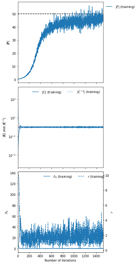
Note we know the analytic value of the determinant of the Fisher information for this problem (\(|\bf{F}|=50\)) so we can add this line to the plot too, and save the output as a png named history_plot.

Parameters

ax (mpl.axes or None, default=None) – An axes object of predefined axes to be labelled
expected_detF (float or None, default=None) – Value of the expected determinant of the Fisher information to plot a horizontal line at to check fitting progress
colour (str or rgb/a value or list, default="C0") – Colour to plot the lines
figsize (tuple, default=(5, 15)) – The size of the figure to be produced
label (str, default="") – Name to add to description in legend
filename (str or None, default=None) – Filename to save plot to
ncol (int, default=1) – Number of columns to have in the legend

Returns

An axes object of the filled plot

Return type

mpl.axes

set_F_statistics(w=None, key=None, validate=True)¶

Set necessary attributes for calculating score compressed summaries

Parameters

w (list or None, default=None) – The network parameters if wanting to calculate the Fisher information with a specific set of network parameters
key (int(2,) or None, default=None) – A random number generator for generating simulations on-the-fly
validate (bool, default=True) – Whether to calculate Fisher information using the validation set

Aggregation of gradients ¶

class imnn.imnn._aggregated_imnn._AggregatedIMNN(host, devices, n_per_device)¶

Manual aggregation of gradients for the IMNN parent class

This class defines the overriding fitting functions for _IMNN() which allows gradients to be aggregated manually. This is necessary if networks or input data are extremely large (or if the number of simulations necessary to estimate the covariance of network outputs, n_s, is very large) since all operations may not fit in memory.

The aggregation is done by calculating n_per_device network outputs at once on each available jax.device() and then scanning over all n_s inputs and n_d simulations necessary to calculate the derivative of the mean of the network outputs with respect to the model parameters. This gives a set of summaries and derivatives from which the loss function

\[\Lambda = -\log|\bf{F}| + r(\Lambda_2) \Lambda_2\]

(See IMNN: Information maximising neural networks) can be calculated and its gradient with respect to these summaries, \(\frac{\partial\Lambda}{\partial x_i^j}\) and derivatives \(\frac{\partial\Lambda}{\partial\partial{x_i^j}/ \partial\theta_\alpha}\) calculated, where \(i\) labels the network output and \(j\) labels the simulation. Note that these are small in comparison to the gradient with respect to the network parameters since their sizes are n_s * n_summaries and n_d * n_summaries * n_params respectively. Once \(\frac{\partial\Lambda}{\partial{x_i^j}}\) and \(\frac{\partial\Lambda}{\partial\partial{x_i^j}/\partial \theta_\alpha}\) are calculated then gradients of the network outputs with respect to the network parameters \(\frac{\partial{x_i^j}}{\partial{w_{ab}^l}}\) and \(\frac{\partial\partial{x_i^j}/\partial\theta_\alpha} {\partial{w_{ab}^l}}\) are calculated and the chain rule is used to get

\[\frac{\partial\Lambda}{\partial{w_{ab}^l}} = \frac{\partial \Lambda}{\partial{x_i^j}}\frac{\partial{x_i^j}} {\partial{w_{ab}^l}} + \frac{\partial\Lambda} {\partial\partial{x_i^j}/\partial\theta_\alpha} \frac{\partial\partial{x_i^j}/\partial\theta_\alpha} {\partial{w_{ab}^l}}\]

Note that we keep the memory use low because only n_per_device simulations are handled at once before being summed into a single gradient list on each device.

n_per_devices should be as large as possible to get the best performance. If everything will fit in memory then this class should be avoided.

The AttributedIMNN class doesn’t directly inherit from _IMNN(), but is meant to be built within a child class of it. For this reason there are attributes which are not explicitly set here, but are used within the module. These will be noted in Other Parameters below.

Parameters

host (jax.device) – The main device where the Fisher information calculation is performed
devices (list) – A list of the available jax devices (from jax.devices())
n_devices (int) – Number of devices to aggregated calculation over
n_per_device (int) – Number of simulations to handle at once, this should be as large as possible without letting the memory overflow for the best performance

model:: Neural network as a function of network parameters and inputs

_get_parameters:: Function which extracts the network parameters from the state

_model_initialiser:: Function to initialise neural network weights from RNG and shape tuple

_opt_initialiser:: Function which generates the optimiser state from network parameters

_update:: Function which updates the state from a gradient

batch_summaries:: Jitted function to calculate summaries on each XLA device

batch_summaries_with_derivatives:: Jitted function to calculate summaries from derivative on each device

batch_gradients:: Jitted function to calculate gradient on each XLA device

batch_gradients_with_derivatives:: Jitted function to calculate gradient from derivative on eachdevice

Public Methods:

`__init__`(host, devices, n_per_device)	Constructor method
`fit`(λ, ε[, rng, patience, min_iterations, …])	Fitting routine for the IMNN
`get_summaries`(w[, key, validate])	Gets all network outputs and derivatives wrt model parameters
`get_gradient`(dΛ_dx, w[, key])	Aggregates gradients together to update the network parameters

Private Methods:

`_set_devices`(devices, n_per_device)	Checks that devices exist and that reshaping onto devices can occur
`_set_batch_functions`()	Creates jitted functions placed on desired XLA devices
`_set_shapes`()	Calculates the shapes for batching over different devices
`_setup_progress_bar`(print_rate, max_iterations)	Construct progress bar
`_update_progress_bar`(pbar, counter, …[, close])	Updates (and closes) progress bar
`_collect_input`(key[, validate])	Returns the dataset to be interated over
`_get_batch_summaries`(inputs, w, θ[, …])	Vectorised batch calculation of summaries or gradients
`_split_dΛ_dx`(dΛ_dx)	Separates dΛ_dx and d2Λ_dxdθ and reshapes them for aggregation
`_construct_gradient`(layers[, aux, func])	Multiuse function to iterate over tuple of network parameters

_collect_input(key, validate=False)¶

Returns the dataset to be interated over

Parameters

key (int(2,)) – A random number generator
validate (bool, default=False) – Whether to use the validation set or not

_construct_gradient(layers, aux=None, func='zeros')¶

Multiuse function to iterate over tuple of network parameters

The options are:

"zeros" – to create an empty gradient array
"einsum" – to combine tuple of dx_dw with dΛ_dx
"derivative_einsum" – to combine tuple of d2x_dwdθ with d2Λ_dxdθ
"sum" – to reduce sum batches of gradients on the first axis

Parameters

layers (tuple) – The tuple of tuples of arrays to be iterated over
aux (float(various shapes)) – parameter to pass dΛ_dx and d2Λ_dxdθ to einsum
func (str) –
Option for the function to apply
- "zeros" – to create an empty gradient array
- "einsum" – to combine tuple of dx_dw with dΛ_dx
- "derivative_einsum" – to combine tuple of d2x_dwdθ with d2Λ_dxdθ
- "sum" – to reduce sum batches of gradients on the first axis

Returns

Tuple of objects like the gradient of the loss function with respect to the network parameters

Return type

tuple

Raises

ValueError – If applied function is not implemented

_get_batch_summaries(inputs, w, θ, gradient=False, derivative=False)¶

Vectorised batch calculation of summaries or gradients

Parameters

inputs (tuple) –
- dΛ_dx if gradient (float(n_per_device, n_summaries) or tuple)
  - dΛ_dx (float(n_per_device, n_summaries)) – The gradient of the loss function with respect to network outputs
  - d2Λ_dxdθ if derivative (float(n_per_device, n_summaries, n_params)) – The gradient of the loss function with respect to derivative of network outputs with respect to model parameters
- keys if SimulatorIMNN() (int(n_per_device, 2)) – The keys for generating simulations on-the-fly
- d if NumericalGradientIMNN() (float(n_per_device, input_shape) or tuple)
  - d (float(n_per_device, input_shape)) – The simulations to be evaluated
  - dd_dθ if derivative (float(n_per_device, input_shape, n_params)) – The derivative of the simulations to be evaluated with respect to model parameters
w (list) – Network model parameters
θ (float(n_params,)) – The value of the model parameters to generate simulations at/to perform the derivative calculation
gradient (bool) – Whether to do the gradient calculation
derivative (bool, default=False) – Whether the gradient of loss function with respect to the derivative of the network outputs with respect to the model parameters is being used

Returns

x if not gradient (float(n_per_device, n_summaries) or tuple)
- x (float(n_per_device, n_summaries)) – The network outputs
- dd_dθ if derivative (float(n_per_device, n_summaries, n_params)) – The derivative of the network outputs with respect to model parameters
if gradient
(tuple) – The accumlated and aggregated gradient of the loss function with respect to the network parameters

Return type

float(n_devices, n_per_device, n_summaries) or tuple

_set_batch_functions()¶

Creates jitted functions placed on desired XLA devices

For each set of summaries to correctly be calculated on a particular device we predefine the jitted functions on each of these devices

_set_devices(devices, n_per_device)¶

Checks that devices exist and that reshaping onto devices can occur

Due to the aggregation then balanced splits must be made between the different devices and so these are checked.

Parameters

devices (list) – A list of the available jax devices (from jax.devices())
n_per_device (int) – Number of simulations to handle at once, this should be as large as possible without letting the memory overflow for the best performance

Raises

ValueError – If devices or n_per_device are None
ValueError – If balanced splitting cannot be done
TypeError – If devices is not a list and if n_per_device is not an int

_set_shapes()¶

Calculates the shapes for batching over different devices

Not implemented

Raises: ValueError – Not implemented in _AggregatedIMNN

_setup_progress_bar(print_rate, max_iterations)¶

Construct progress bar

Parameters

print_rate (int or None) – The rate at which the progress bar is updated (no bar if None)
max_iterations (int) – The maximum number of iterations, used to setup bar upper limit

Returns

progress bar or None – The TQDM progress bar object
int or None – The print rate (after checking for int or None)
int or None – The difference between the max_iterations and the print rate

Raises

TypeError: – If print_rate is not an integer

_split_dΛ_dx(dΛ_dx)¶

Separates dΛ_dx and d2Λ_dxdθ and reshapes them for aggregation

Parameters

dΛ_dx (tuple) –

dΛ_dx (float(n_s, n_summaries)) – The derivative of the loss function wrt the network outputs
d2Λ_dxdθ (float(n_d, n_summaries, n_params)) – The derivative of the loss function wrt the derivative of the network outputs wrt the model parameters

Raises

ValueError – function not implemented in parent class

_update_progress_bar(pbar, counter, patience_counter, max_detF, detF, detC, detinvC, Λ2, r, print_rate, max_iterations, remainder, close=False)¶

Updates (and closes) progress bar

Checks whether a pbar is used and is so checks whether the iteration coincides with the print rate, or is the last set of iterations within the print rate from the last iteration, or if the last iteration has been reached and the bar should be closed.

Parameters

pbar (progress bar object) – The TQDM progress bar
counter (int) – The value of the current iteration
patience_counter (int) – The number of iterations where the maximum of the determinant of the Fisher information matrix has not increased
max_detF (float) – Maximum of the determinant of the Fisher information matrix
detF (float(n_params, n_params)) – Fisher information matrix
detC (float(n_summaries, n_summaries)) – Covariance of the network summaries
detinvC (float(n_summaries, n_summaries)) – Inverse covariance of the network summaries
Λ2 (float) – Value of the regularisation term
r (float) – Value of the dynamic regularisation coupling strength
print_rate (int or None) – The number of iterations to run before updating the progress bar
max_iterations (int) – The maximum number of iterations to run
remainder (int or None) – The number of iterations before max_iterations to check progress
close (bool, default=False) – Whether to close the progress bar (on final iteration)

fit(λ, ε, rng=None, patience=100, min_iterations=100, max_iterations=100000, print_rate=None, best=True)¶

Fitting routine for the IMNN

Parameters

λ (float) – Coupling strength of the regularisation
ϵ (float) – Closeness criterion describing how close to the 1 the determinant of the covariance (and inverse covariance) of the network outputs is desired to be
rng (int(2,) or None, default=None) – Stateless random number generator
patience (int, default=10) – Number of iterations where there is no increase in the value of the determinant of the Fisher information matrix, used for early stopping
min_iterations (int, default=100) – Number of iterations that should be run before considering early stopping using the patience counter
max_iterations (int, default=int(1e5)) – Maximum number of iterations to run the fitting procedure for
print_rate (int or None, default=None,) – Number of iterations before updating the progress bar whilst fitting. There is a performance hit from updating the progress bar more often and there is a large performance hit from using the progress bar at all. (Possible RET_CHECK failure if print_rate is not None when using GPUs). For this reason it is set to None as default
best (bool, default=True) – Whether to set the network parameter attribute self.w to the parameter values that obtained the maximum determinant of the Fisher information matrix or the parameter values at the final iteration of fitting

Example

We are going to summarise the mean and variance of some random Gaussian noise with 10 data points per example using an AggregatedSimulatorIMNN. In this case we are going to generate the simulations on-the-fly with a simulator written in jax (from the examples directory). These simulations will be generated on-the-fly and passed through the network on each of the GPUs in jax.devices("gpu") and we will make 100 simulations on each device at a time. The main computation will be done on the CPU. We will use 1000 simulations to estimate the covariance of the network outputs and the derivative of the mean of the network outputs with respect to the model parameters (Gaussian mean and variance) and generate the simulations at a fiducial μ=0 and Σ=1. The network will be a stax model with hidden layers of [128, 128, 128] activated with leaky relu and outputting 2 summaries. Optimisation will be via Adam with a step size of 1e-3. Rather arbitrarily we’ll set the regularisation strength and covariance identity constraint to λ=10 and ϵ=0.1 (these are relatively unimportant for such an easy model).

import jax
import jax.numpy as np
from jax.experimental import stax, optimizers
from imnn import AggregatedSimulatorIMNN

rng = jax.random.PRNGKey(0)

n_s = 1000
n_d = 1000
n_params = 2
n_summaries = 2
input_shape = (10,)
θ_fid = np.array([0., 1.])

def simulator(rng, θ):
    return θ[0] + jax.random.normal(
        rng, shape=input_shape) * np.sqrt(θ[1])

model = stax.serial(
    stax.Dense(128),
    stax.LeakyRelu,
    stax.Dense(128),
    stax.LeakyRelu,
    stax.Dense(128),
    stax.LeakyRelu,
    stax.Dense(n_summaries))
optimiser = optimizers.adam(step_size=1e-3)

λ = 10.
ϵ = 0.1

model_key, fit_key = jax.random.split(rng)

host = jax.devices("cpu")[0]
devices = jax.devices("gpu")

n_per_device = 100

imnn = AggregatedSimulatorIMNN(
    n_s=n_s, n_d=n_d, n_params=n_params, n_summaries=n_summaries,
    input_shape=input_shape, θ_fid=θ_fid, model=model,
    optimiser=optimiser, key_or_state=model_key,
    simulator=simulator, host=host, devices=devices,
    n_per_device=n_per_device)

imnn.fit(λ, ϵ, rng=fit_key, min_iterations=1000, patience=250,
         print_rate=None)

Notes

A minimum number of interations should be be run before stopping based on a maximum determinant of the Fisher information achieved since the loss function has dual objectives. Since the determinant of the covariance of the network outputs is forced to 1 quickly, this can be at the detriment to the value of the determinant of the Fisher information matrix early in the fitting procedure. For this reason starting early stopping after the covariance has converged is advised. This is not currently implemented but could be considered in the future.

The best fit network parameter values are probably not the most representative set of parameters when simulating on-the-fly since there is a high chance of a statistically overly-informative set of data being generated. Instead, if using fit() consider using best=False which sets self.w=self.final_w which are the network parameter values obtained in the last iteration. Also consider using a larger patience value if using fit() to overcome the fact that a flukish high value for the determinant might have been obtained due to the realisation of the dataset.

Raises

TypeError – If any input has the wrong type
ValueError – If any input (except rng) are None
ValueError – If rng has the wrong shape
ValueError – If rng is None but simulating on-the-fly

get_keys_and_params:: Jitted collection of parameters and random numbers

calculate_loss:: Returns the jitted gradient of the loss function wrt summaries

validation_loss:: Jitted loss and auxillary statistics from validation set

get_gradient(dΛ_dx, w, key=None)¶

Aggregates gradients together to update the network parameters

To avoid having to calculate the gradient with respect to all the simulations at once we aggregate by addition the gradient calculation by looping over the simulations again and combining them with the derivative of the loss function with respect to the network outputs (and their derivatives with respect to the model parameters). Whilst this is expensive, it is necessary since we cannot make a stochastic estimate of the Fisher information accurately and therefore we need to use all the simulations available - which is probably too large to fit in memory.

Parameters

dΛ_dx (tuple) –
- dΛ_dx float(n_s, n_params, n_summaries) – the derivative of the loss function with respect to network summaries
- d2Λ_dxdθ float(n_d, n_summaries, n_params) – the derivative of the loss function with respect to the derivative of network summaries with respect to model parameters
w (list) – Network parameters
key (None or int(2,)) – Random number generator used in SimulatorIMNN

Returns

The gradient of the loss function with respect to the network parameters calculated by aggregating

Return type

list

Raises

ValueError – function not implemented in parent class

get_summaries(w, key=None, validate=False)¶

Gets all network outputs and derivatives wrt model parameters

Parameters

w (list or None, default=None) – The network parameters if wanting to calculate the Fisher information with a specific set of network parameters
key (int(2,) or None, default=None) – A random number generator for generating simulations on-the-fly
validate (bool, default=True) – Whether to get summaries of the validation set

Returns

float(n_s, n_summaries) – The network outputs
float(n_d, n_summaries, n_params) – The derivative of the network outputs wrt the model parameters

Raises

ValueError – function not implemented in parent class

Parent classes¶

Base class ¶

Aggregation of gradients ¶

Information Maximising Neural Network

Navigation

Related Topics

Parent classes¶

Base class¶

Aggregation of gradients¶

Base class ¶

Aggregation of gradients ¶